Survey design simulation (DSsim) case study
Author: Laura Marshall
library(knitr)
library(DSsim)
This case study shows you how to use the R package DSsim (Marshall 2014) to compare the performance of different survey designs. We will replicate the analyses of Sections 3.5.2 and 12.1.1 of the book.
1 Getting started
Ensure you have administrator privileges on your computer and install the necessary R packages.
needed.packages <- c("DSsim", "mrds", "shapefiles", "splancs")
myrepo <- "http://cran.rstudio.com"
install.packages(needed.packages, repos = myrepo)
1.1 Directory structure for files in this project
Examine the other files and folders in the “DSsim_ study” folder. There are three files starting with the name “Region” and ending with .dbf, .shp and .shx, these files make up the shapefile for the survey region. The density.surface.robj file is the density surface for the survey region. The Survey Transects folder contains a folder for each of the designs you are asked to look at, these contain the transect shapefiles. The Results folder contains the results from 999 replications as this can take a good few hours to run. Select the directory that contains these files.
The DSsim Example Distance project is included so you can view the specification of the designs if you wish, or you could even have a go at testing out a new design.
2 Creating a new simulation
2.1 Creating a region object
Read the Region shapefile into R.
library(shapefiles)
region.shapefile <- read.shapefile("DSsim_study/Region")
Next create the region object using this shapefile. As there are no strata in this example, you just need to provide a name for your survey region and specify the units (metres, m).
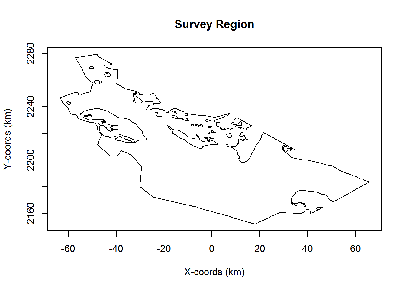
region <- make.region(region.name = "Survey Region", units = "m", shapefile = region.shapefile)View the resulting object:
plot(region, plot.units = "km")
2.2 Creating a density object
Now create a density object within this region. For this study, a density surface has already been created, but you can experiment with the options in the next code chunk to define one yourself.
You can create other density surfaces by creating a density object based on a uniform density grid over the area, and adding some hot spots (or low spots).
density <- make.density(region = region, x.space = 1000, y.space = 1000, constant = 4e-08)
density <- add.hotspot(density, centre = c(-2500, 2224000), sigma = 10000, amplitude = 1e-08)
density <- add.hotspot(density, centre = c(0, 2184000), sigma = 18000, amplitude = -5e-09)
Load the density surface and view the data that comprise the surface.
load("DSsim_study/density.surface.robj")
kable(density.surface[[1]][1:5, ])| x | y | density |
|---|---|---|
| 17071.09 | 2152699 | 1e-07 |
| 18071.09 | 2152699 | 1e-07 |
| 15071.09 | 2153699 | 1e-07 |
| 16071.09 | 2153699 | 1e-07 |
| 17071.09 | 2153699 | 1e-07 |
The density surface is a data set of x and y locations and corresponding densities at each point.
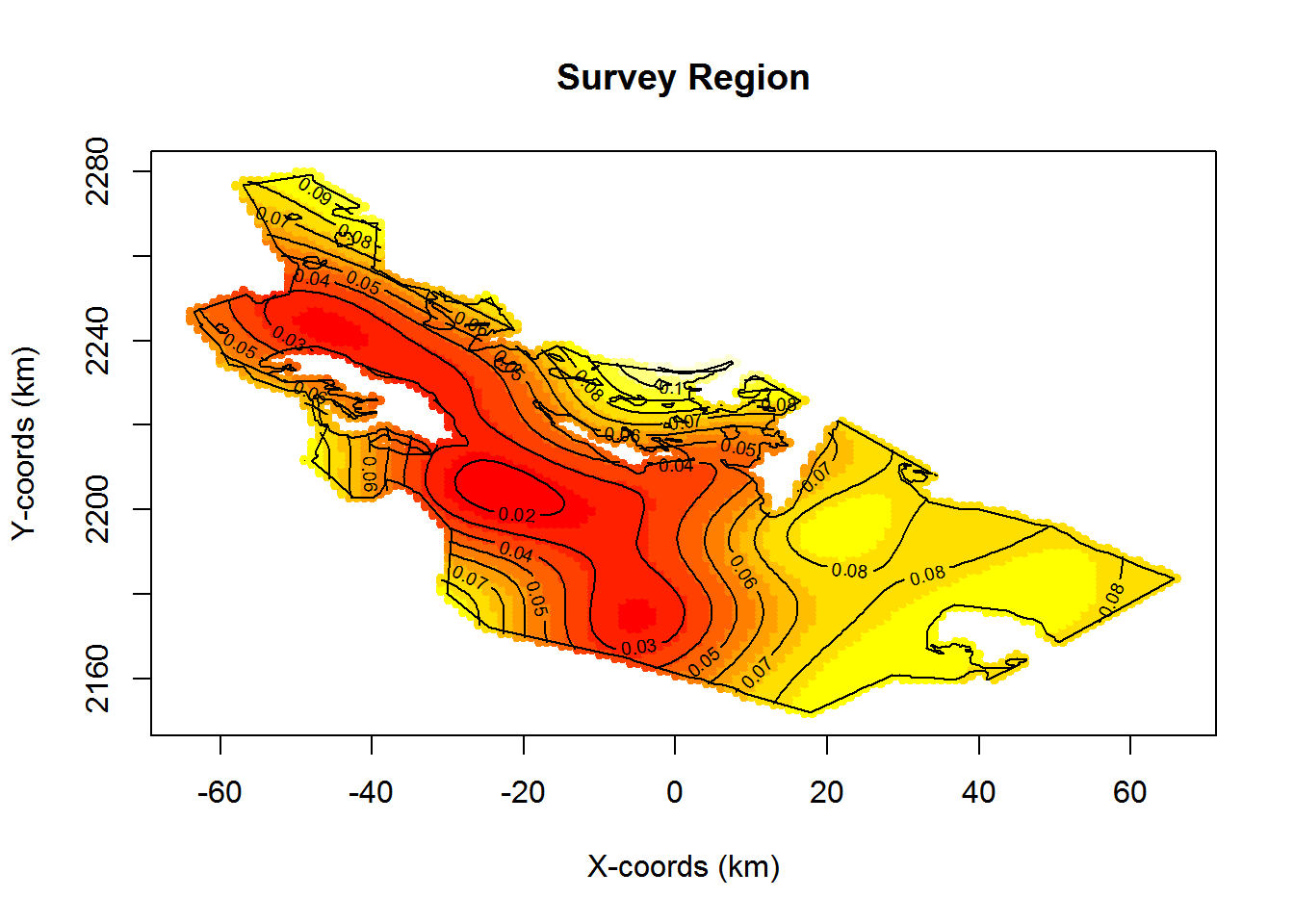
To create the density object, you need to provide the density surface, the region object for which it was created, and the grid spacing that was used. I used a grid spacing of 1000m in both the x and y directions to create this density surface.
pop.density <- make.density(region = region, density.surface = density.surface,
    x.space = 1000, y.space = 1000)
View the density surface.
plot(pop.density, plot.units = "km")
plot(region, add = TRUE)
2.2.1 Population size
Fix the population size at 1500 individuals. Using make.population.description set the first argument to the desired population abundance and set the second argument such that exactly this number of individuals is generated in each realisation (fixed.N = TRUE).
pop.description <- make.population.description(region.obj = region, density.obj = pop.density,
    N = 1500, fixed.N = TRUE)
2.2.2 True detection function
We select a half-normal detection function with a /sigma/sigma (scale.param) of 500m and a truncation distance of 1000m.
detect <- make.detectability(key.function = "hn", scale.param = 500, truncation = 1000)2.3 Creating the survey design object
We first consider the subjective design (Section 12.1.1 of the book). The subjective design uses existing paths together with additional transects chosen to achieve a more even coverage of the survey region.
NOTE: you will need to edit the path argument to describe where the files are on your machine. Look back to the path you found when you were setting up and add “/Survey Transects/Subjective Design”.
new.directory <- paste(getwd(), "DSsim_study/Survey_Transects/Subjective_Design",
    sep = "/")
subjective.design <- make.design(transect.type = "Line", design.details = c("user specified"),
    region = region, plus.sampling = FALSE, path = new.directory)
subjective.design@filenames
[1] "New_Des1"Previous code not only constructs the subjective design, but prints out the names of the shapefiles that will be used in the simulation. This is a check that the working directory has been set properly. The command subjective.design@filenames is a check to make sure the correct folder has been identified. This will tell you the names of the shapefiles the simulation will use.
2.4 Creating the analyses object
Describe the analyses to carry out on the simulated data. Here we propose both half-normal and hazard-rate models (neither with covariates) and choose between them based on the AIC values.
ddf.analyses <- make.ddf.analysis.list(
        dsmodel = list(~cds(key = "hn", formula = ~1), #half-normal model
        ~cds(key = "hr", formula = ~1)),               #hazard-rate model
        method = "ds", criteria = "AIC")
2.5 Creating the simulation object
We can finally put it all together and have a look at some example populations, transects and survey data. Set the number of repetitions (reps) to be fairly low initially to avoid long run times. For the subjective design, specify that the same set of transects is to be used in each replicate, single.transect.set = TRUE.
my.simulation.subjective <- make.simulation(reps = 10, single.transect.set = TRUE,
    region.obj = region, design.obj = subjective.design, population.description.obj = pop.description,
    detectability.obj = detect, ddf.analyses.list = ddf.analyses)
Before running the simulation, you can check to see that it is doing what you want. These commands will allow you to investigate the simulation properties.
# set the display window up for 4 plots
par(mfrow = c(2, 2))
# generate and plot and example population
pop <- generate.population(my.simulation.subjective)
plot(region)
plot(pop)
# generate (or rather load from file) the transects
transects <- generate.transects(my.simulation.subjective)
plot(region)
plot(transects, col = 4, lwd = 2)
# simulate the survey process of detection
eg.survey <- create.survey.results(my.simulation.subjective)
plot(eg.survey)
# have a look at the distance data from the simulated survey
dist.data <- get.distance.data(eg.survey)
hist(dist.data$distance, xlab = "Distance (m)", main = "Distance Data")
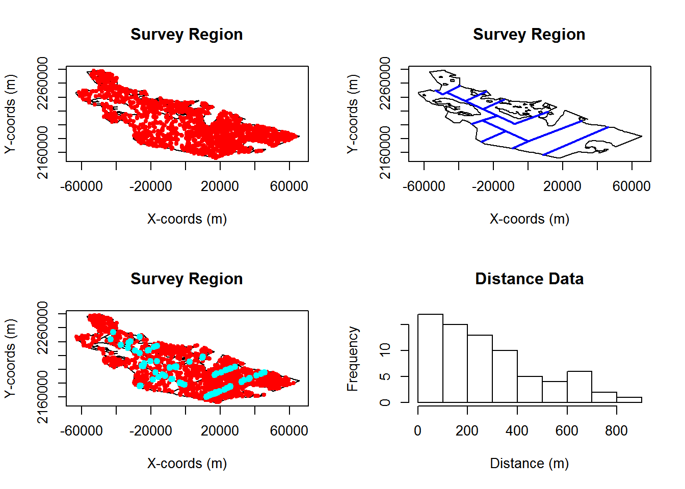
par(mfrow = c(1, 1))If the previous plots lead you to believe you have properly parameterised your simulation, it is time to run it. Be patient, as it will take a few minutes to complete.
my.simulation.subjective.run <- run(my.simulation.subjective)Information about effort, estimated abundance, estimated density and detection probability (Pa)(Pa) is available in the resulting object. Results from each replicate for abundance estimation can be examined, such as
kable(t(my.simulation.subjective.run@results$individuals$N[, , 5]), digits = 3,
caption = "Estimate of abundance (with measures of precision) for the fifth replicate of the simulation performed above.")| Estimate | se | cv | lcl | ucl | df |
|---|---|---|---|---|---|
| 1234.838 | 363.637 | 0.294 | 666.922 | 2286.36 | 14.631 |
or average abundance estimates across replicates
kable(t(my.simulation.subjective.run@results$individuals$N[, , 11]), digits = 3,
caption = "Average estimate of abundance (with measures of precision) across all replicates of the simulation performed above.")| Estimate | se | cv | lcl | ucl | df |
|---|---|---|---|---|---|
| 1087.524 | 263.772 | 0.241 | 660.672 | 1809.086 | 19.605 |
There is also a summary() function for simulation results objects that provide more exhaustive results.
3 On to randomised designs
You will need to create 2 new simulations each with a new design object, one for the parallel design and one for the zigzag design. The other objects (region, density, population description etc.) should be left the same. Here is how to do it for the parallel design (path directed to folder containing shape files associated with a parallel transect survey design).
Note: We now wish different transects to be used on each repetition (single.transect.set = FALSE).
parallel.directory <- paste(getwd(), "DSsim_study/Survey_Transects/Parallel_Design",
    sep = "/")
parallel.design <- make.design(transect.type = "Line", design.details = c("Parallel",
    "Systematic"), region.obj = region, design.axis = 45, spacing = 12000, plus.sampling = FALSE,
    path = parallel.directory)
my.simulation.parallel <- make.simulation(reps = 10, single.transect.set = FALSE,
    region.obj = region, design.obj = parallel.design, population.description.obj = pop.description,
    detectability.obj = detect, ddf.analyses.list = ddf.analyses)
The code does not complete the process of analysing and summarising the simulation of systematic parallel line transects. The user can complete this investigation.
3.1 Contrast bias and precision from subjective and randomised surveys
More than 10 replicates are needed to adequately address the question of bias. Results of a more extensive simulation study are stored as workspace objects. The following code loads these results.
load("DSsim_study/Results/simulation.subjective.robj")
load("DSsim_study/Results/simulation.parallel.robj")
load("DSsim_study/Results/simulation.zigzag.robj")
We can extract components from these R objects to approximate the findings presented in Table 2.1, page 29 of the book.
extract.metrics <- function(simobj) {
    nreps <- simobj@reps
    data <- simobj@results$individuals$summary
    effort.avg <- data[, , nreps + 1][3]/1000
    detects.avg <- data[, , nreps + 1][4]
    abund <- simobj@results$individuals$N
    abund.avg <- abund[, , nreps + 1][1]
    true.N <- [email protected]@N
    est.bias <- (abund.avg - true.N)/true.N
    est.bias.pct <- est.bias * 100
    mean.stderr <- abund[, , nreps + 1][2]
    stddev <- abund[, , nreps + 2][1]
    result.vector <- unname(c(effort.avg, detects.avg, abund.avg, est.bias.pct,
        mean.stderr, stddev))
    return(result.vector)
}
subjective <- extract.metrics(simulation.subjective)
parallel <- extract.metrics(simulation.parallel)
zigzag <- extract.metrics(simulation.zigzag)

result.table <- data.frame(subjective, parallel, zigzag, row.names = c("Mean effort(km)",
    "Mean sample size", "Mean abundance estimate", "Estimated percent bias",
    "Mean SE of abundance estimate", "SD of abundance estimates"))
kable(result.table, digits = 1, caption = "Simulation results summary for each design. Estimates based upon 999 simulations with true abundance of 1500 objects.")| subjective | parallel | zigzag | |
|---|---|---|---|
| Mean effort(km) | 336.8 | 473.5 | 694.6 |
| Mean sample size | 85.0 | 146.5 | 215.2 |
| Mean abundance estimate | 1214.5 | 1484.5 | 1480.2 |
| Estimated percent bias | -19.0 | -1.0 | -1.3 |
| Mean SE of abundance estimate | 283.4 | 216.2 | 173.6 |
| SD of abundance estimates | 225.0 | 193.9 | 154.9 |
References
Marshall, L. 2014. DSsim: Distance sampling simulations.