Montrave songbird case study in R
Case studies, 2 September 2015
1 Analysis of robin line transect data
library(Distance)
library(knitr)
1.1 Reading line transect data from a CSV file
This is a one-line operation.
birds.line <- read.csv("montrave-line.csv")1.2 Massaging the data
This is more challenging, because of two ideosyncracies of this survey.
1.2.1 Multiple walks of transects
Prof. Buckland walked each of the transects twice. This must be taken into account in the analysis, lest the density estimates be too high by a factor of two. In the Distance GUI project, there is a column labelled visitsin the Study area layer. This treats visits as a multiplier applied to all transect line lengths. I have chosen a different option here, and I have simply multiplied the column Effort by the column I have relabelled repeats.
birds.line$Effort <- birds.line$Effort * birds.line$repeats1.2.2 Filtering by species
A more challenging set of alteration to the data is to analyse data for a single species. You may recall that during the Montrave survey, Prof. Buckland recorded detections of a number of species; we wish here to only analyse data for robins. It is quite simple to select only the records describing detections of robins. That can be accomplished either with the subset function, or by specifying a test condition that will retain rows of the data frame that match that condition. I show both.
A much stickier problem is created by this filtering by species. The problem is that some transects may not have had detections of the species of interest. The effort associated with all transects (whether or not robins were detected) need to be included in the analysis, otherwise density will be estimated improperly because survey effort is not carried forward after filtering out only detections of robins.
The code below determines line lengths for all transects, determines whether any transects failed to have robin detections (3 of 19 transects did not have robin detections). Line lengths for those 3 transects are appended onto the robins data frame. The data frame is sorted by Sample.Label such that the empty transects appear in the proper sequence in the data frame.
robins <- birds.line[birds.line$species=="r", ]
# robins <- subset(birds.line,  species=="r") # is equivalent

# http://stackoverflow.com/questions/13765834/r-equivalent-of-first-or-last-sas-operator
  findFirstLast <- function(myDF, findFirst=TRUE) {
  # myDF should be a data frame or matrix
    # By default, this function finds the first occurence of each unique value in a column
    # If instead we want to find last, set findFirst to FALSE.
    # This will give `maxOrMin` a value of -1 finding the min of the negative indexes
    # is the same as finding the max of the positive indexes
    maxOrMin <- ifelse(findFirst, 1, -1)
    # For each column in myDF, make a list of all unique values (`levs`) and
    # iterate over that list, finding the min (or max) of all the indexes
    # of where that given value appears within the column
    apply(myDF, 2, function(colm) {
        levs <- unique(colm)
        sapply(levs, function(lev) {
          inds <- which(colm==lev)
          ifelse(length(inds)==0, NA, maxOrMin*min(inds*maxOrMin) )
        })
      })
  }
tran.with.robins <- unique(robins$Sample.Label) # transect IDs with robins
all.trans <- seq(1: length(unique(birds.line$Sample.Label))) # transect IDs all transects
# empty transects will occupy the last few elements of the union statement
empty.transects <- union(tran.with.robins,
                         all.trans)[(length(tran.with.robins)+1):length(all.trans)]
#  what are the lengths of those empty transects?
all.transect.lengths <- findFirstLast(birds.line)$Sample.Label
lengths.empty.transects <- birds.line$Effort[all.transect.lengths[empty.transects]]
# append 'blank' rows to bottom of species-specific data set
# retain effort of transects with no sightings
empty <- NULL
for (i in 1:length(empty.transects)) {
   blank <- cbind(birds.line[1,1:3], empty.transects[i], lengths.empty.transects[i])
   empty <- rbind(empty, blank)
}
empty[,c("A","B","C")] <- NA  # pad out columns that are blank (distance, species, visit)
names(empty) <- names(birds.line)
robins <- rbind(robins, empty)
robins <- robins[order(robins$Sample.Label), ]
1.3 Detection function fitting for line transect data
Only a small number of models are fitted to these data (matching those models fitted in the Distance GUI):
robin.hn.herm <- ds(robins, truncation=95, transect="line",
                    key="hn", adjustment="herm", convert.units=.1)
robin.uni.cos <- ds(robins, truncation=95, transect="line",
                    key="unif", adjustment="cos", convert.units=.1)
robin.haz.simp <- ds(robins, truncation=95, transect="line",
                    key="hr", adjustment="poly", convert.units=.1)
model.results <- rbind(robin.uni.cos$dht$individuals$D, robin.haz.simp$dht$individuals$D,
                       robin.hn.herm$dht$individuals$D)
1.4 Goodness of fit for line transect data
robin.breaks <- c(0,12.5,22.5,32.5,42.5,52.5,62.5,77.5,95) # from Distance GUI
fit.uni.cos <- ddf.gof(robin.uni.cos$ddf, breaks=robin.breaks,
                       main="Montrave robin line transect data, Uniform-cosine detection function")
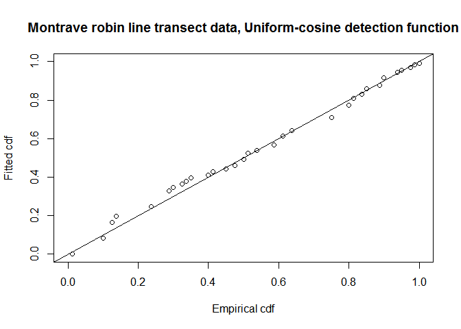 QQ-plot of uniform cosine model fit to Montrave robin line transect data.
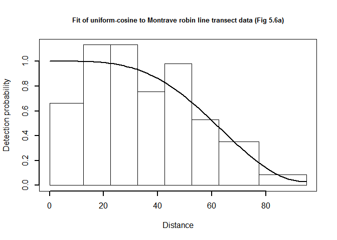
plot(robin.uni.cos$ddf, showpoints=FALSE, pl.den=0, lwd=2, breaks=robin.breaks,
     main="Fit of uniform-cosine to Montrave robin line transect data (Fig 5.6a)")
QQ-plot of uniform cosine model fit to Montrave robin line transect data.
chirow <- c(fit.uni.cos$chisquare$chi1$chisq, fit.uni.cos$chisquare$chi1$p)
ksrow <- c(fit.uni.cos$dsgof$ks$Dn, fit.uni.cos$dsgof$ks$p)
cvmrow <- c(fit.uni.cos$dsgof$CvM$W, fit.uni.cos$dsgof$CvM$p)
mytable <- rbind(chirow, ksrow, cvmrow)
rownames(mytable) <- c("Chi-square test", "K-S test", "CvM test")
kable(mytable, col.names = c("Test statistic", "P-value"), digits=3,
caption="Goodness of fit statistics, Montrave robin line transects, Uniform-cosine model")| Test statistic | P-value | |
|---|---|---|
| Chi-square test | 3.804 | 0.578 |
| K-S test | 0.111 | 0.281 |
| CvM test | 0.117 | 0.510 |
1.5 Report density estimates for line transect data
There is little to choose between fitted models, based upon either AIC or goodness of fit. We present the density estimates and measures of precision for the three models fitted to the robin line transect data.
# Inelegant way to build first column model names
model.results[,1] <- as.character(model.results[,1])
model.results[1,1] <- "Unif.cosine"
model.results[2,1] <- "Hazard rate"
model.results[3,1] <- "Half-norm. Hermite"
kable(model.results[,1:6], digits=3,
caption="Density estimates under Uniform/cos, Hazard rate, and half-normal Hermite models (Table 6.3).")| Label | Estimate | se | cv | lcl | ucl |
|---|---|---|---|---|---|
| Unif.cosine | 0.686 | 0.132 | 0.192 | 0.470 | 1.001 |
| Hazard rate | 0.642 | 0.083 | 0.129 | 0.495 | 0.832 |
| Half-norm. Hermite | 0.696 | 0.153 | 0.219 | 0.453 | 1.071 |
2 Analysis of robin point transect data
The analysis of Montrave robin point count data mimics the analysis of robin line transect data: read data, filter by species, fit detection functions, assess fit, report results.
2.1 Reading point transect data from a CSV file
This is a one-line operation.
birds.point <- read.csv("montrave-point.csv")2.2 Massaging the data
As with transect data, filter for the species of interest. Note that in Table 1.2 of Buckland et al. (2015), there are 8 of the 32 transects without robin detections. The code below makes use of the function findFirstLast() used with the line transect data to include effort of the points that had no detections. In this survey, all points were visited two times, so this code is over-engineered to locate the effort associated with the points without detections. But the code provided can cope with the case in which not all points are visited an equal number of times.
robins.pt <- subset(birds.point, species=="r")
pt.with.robins <- unique(robins.pt$Sample.Label) # point IDs with robins
all.points <- seq(1: length(unique(birds.point$Sample.Label))) # point IDs all transects
# empty points will occupy the last few elements of the union statement
empty.points <- union(pt.with.robins, all.points)[(length(pt.with.robins)+1):length(all.points)]
#  what was effort on empty points?
all.point.effort <- findFirstLast(birds.point)$Sample.Label
effort.empty.points <- birds.point$Effort[all.point.effort[empty.points]]
# append 'blank' rows to bottom of species-specific data set
# retain effort of transects with no sightings
empty <- NULL
for (i in 1:length(empty.points)) {
   blank <- cbind(birds.point[1,1:2], empty.points[i], effort.empty.points[i])
   empty <- rbind(empty, blank)
}
empty[,c("A","B","C")] <- NA  # pad out columns that are blank (distance, species, visit)
names(empty) <- names(birds.point)
robins.pt <- rbind(robins.pt, empty)
robins.pt <- robins.pt[order(robins.pt$Sample.Label), ]
2.3 Detection function fitting to snapshot point counts
Only a small number of models are fitted to these data (matching those models fitted in the Distance GUI):
robin.pt.hn.herm <- ds(robins.pt, truncation=110, transect="point",
                    key="hn", adjustment="herm", convert.units=.01) # change in conversion
robin.pt.uni.cos <- ds(robins.pt, truncation=110, transect="point",
                    key="unif", adjustment="cos", convert.units=.01)
robin.pt.haz.simp <- ds(robins.pt, truncation=110, transect="point",
                    key="hr", adjustment="poly", convert.units=.01)
pt.model.results <- rbind(robin.pt.uni.cos$dht$individuals$D, robin.pt.haz.simp$dht$individuals$D,
                       robin.pt.hn.herm$dht$individuals$D)
2.4 Goodness of fit for snapshot point counts
robin.breaks <- c(0,22.5,32.5,42.5,52.5,62.5,77.5,110) # from Section 5.2.3.3
fit.pt.haz.simp <- ddf.gof(robin.pt.haz.simp$ddf, breaks=robin.breaks,
                       main="Montrave robin point transect data, hazard rate detection function")
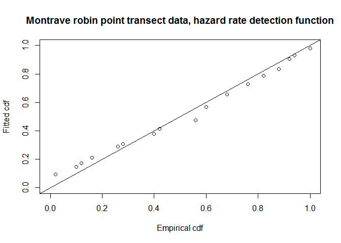
QQ-plot of hazard rate model fit to Montrave robin point transect data.
In addition to the QQ plot, another visual measure of the fit of the model to point count data is the PDF fitted to a histogram of radial detection distances. The function ds has no built-in plotter for the PDF (as does the Distance GUI software). The code below manufactures a PDF plotter and uses it upon the hazard rate model for the robin point count data.
hazard <- function(y, sigma, shape) {
  key <- 1-exp(-(y/sigma)^(-shape))
  return(key)
}
haz <- function(distances, ddfobj, point=TRUE) {
  sigma <- exp(ddfobj$par[2])  # contrary to hn models
  shape <- exp(ddfobj$par[1])
  pr.detect <- hazard(distances, sigma, shape)
  if (point) pr.detect <- pr.detect * distances
  return(pr.detect)
}
pdf.point <- function(ddf.obj, mybreaks, ...) {
#  ddf.obj is produced by a call to ds()
#  result is a plot
#    sort out the pdf
  upperbnd <- ddf.obj$meta.data$int.range[2]
  distances <- seq(0,upperbnd,length.out = 75)
  if (ddf.obj$ds$aux$ddfobj$type=="hn") {
    detfn.line <- hnherm(distances, point=TRUE, ddfobj = ddf.obj)
    df.integral <- integrate(hnherm, lower=0, upper=upperbnd, point=TRUE,
                             ddfobj=ddf.obj)[1]$value
  }
  if (ddf.obj$ds$aux$ddfobj$type=="hr") {
    detfn.line <- haz(distances, point=TRUE, ddfobj=ddf.obj)
    df.integral <- integrate(haz, lower=0, upper=upperbnd, point=TRUE,
                            ddfobj=ddf.obj)[1]$value
  }
  detfn.line <- detfn.line / df.integral
#  now for the bars
  hist.dist <- hist(ddf.obj$data$distance, breaks=mybreaks, plot=FALSE)
#  picture
  plot(hist.dist, freq=FALSE, xlab="Distance", ylab="Probability density",...)
  lines(x=distances, y=detfn.line,...)
  box()
  return(hist.dist)
}
point.plot <- pdf.point(robin.pt.haz.simp$ddf, mybreaks=robin.breaks,
                        main="Montrave robin point counts, hazard pdf", lwd=2)
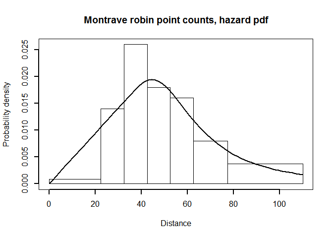
PDF plot of hazard rate fitted to point transect data
chirow <- c(fit.pt.haz.simp$chisquare$chi1$chisq, fit.pt.haz.simp$chisquare$chi1$p)
ksrow <- c(fit.pt.haz.simp$dsgof$ks$Dn, fit.pt.haz.simp$dsgof$ks$p)
cvmrow <- c(fit.pt.haz.simp$dsgof$CvM$W, fit.pt.haz.simp$dsgof$CvM$p)
mytable <- rbind(chirow, ksrow, cvmrow)
rownames(mytable) <- c("Chi-square test", "K-S test", "CvM test")
kable(mytable, col.names = c("Test statistic", "P-value"), digits=3,
caption="Goodness of fit statistics, Montrave robin point transects, hazard rate model")| Test statistic | P-value | |
|---|---|---|
| Chi-square test | 6.390 | 0.172 |
| K-S test | 0.129 | 0.377 |
| CvM test | 0.130 | 0.457 |
2.5 Report density estimates for point transect data
The density estimates can be contrasted with results presented in Section 6.3.1.4 of Buckland et al. (2015).
# Inelegant way to build first column model names
pt.model.results[,1] <- as.character(model.results[,1])
pt.model.results[1,1] <- "Unif.cosine"
pt.model.results[2,1] <- "Hazard rate"
pt.model.results[3,1] <- "Half-norm. Hermite"
kable(pt.model.results[,1:6], digits=3,
caption="Density estimates under Uniform/cos, Hazard rate, and half-normal Hermite models (Table 6.4).")| Label | Estimate | se | cv | lcl | ucl |
|---|---|---|---|---|---|
| Unif.cosine | 0.651 | 0.107 | 0.164 | 0.468 | 0.906 |
| Hazard rate | 0.587 | 0.130 | 0.222 | 0.379 | 0.908 |
| Half-norm. Hermite | 0.786 | 0.181 | 0.231 | 0.499 | 1.237 |
This set of code associated with the Montrave robin data shows the ideosyncracies of contrasting results derived from the Distance GUI with results produced by the R package Distance. With the tips provided herein, interested practicioners can produce roughly comparable results taking either route.